ATLAS empirical electron-muon test

What is relatively new is that this analysis looks at charge and flavor in the hopes of observing a telltale deviation from the standard model.

Miracles when you use the right metric

I recommend reading, carefully and thoughtfully, the preprint “The Metric Space of Collider Events” by Patrick Komiske, Eric Metodiev, and Jesse Thaler (arXiv:1902.02346). There is a lot here, perhaps somewhat cryptically presented, but much of it is exciting.

First, you have to understand what the Earth Mover’s Distance (EMD) is. This is easier to understand than the Wasserstein Metric of which it is a special case. The EMD is a measure of how different two pdfs (probability density functions) are and it is rather different than the usual chi-squared or mean integrated squared error because it emphasizes separation rather than overlap. The idea is look at how much work you have to do to reconstruct one pdf from another, where “reconstruct” means transporting a portion of the first pdf a given distance. You keep track of the “work” you do, which means the amount of area (i.e.,”energy” or “mass”) you transport and how far you transport it. The Wikipedia article aptly makes an analogy with suppliers delivering piles of stones to customers. The EMD is the smallest effort required.

The EMD is a rich concept because it allows you to carefully define what “distance” means. In the context of delivering stones, transporting them across a plain and up a mountain are not the same. In this sense, rotating a collision event about the beam axis should “cost” nothing – i.e, be irrelevant — while increasing the energy or transverse momentum should, because it is phenomenologically interesting.

The authors want to define a metric for LHC collision events with the notion that events that come from different processes would be well separated. This requires a definition of “distance” – hence the word “metric” in the title. You have to imagine taking one collision event consisting of individual particle or perhaps a set of hadronic jets, and transporting pieces of it in order to match some other event. If you have to transport the pieces a great distance, then the events are very different. The authors’ ansatz is a straight forward one, depending essentially on the angular distance θ_ij/R plus a term than takes into account the difference in total energies of the two events. Note: the subscripts i and j refer to two elements from the two different events. The paper gives a very nice illustration for two top quark events (read and blue):

Transformation of one top quark event into another

The first thing that came to mind when I had grasped, with some effort, the suggested metric, was that this could be a great classification tool. And indeed it is. The authors show that a k-nearest neighbors algorithm (KNN), straight out of the box, equipped with their notion of distance, works nearly as well as very fancy machine learning techniques! It is crucial to note that there is no training here, no search for a global minimum of some very complicated objection function. You only have to evaluate the EMD, and in their case, this is not so hard. (Sometimes it is.) Here are the ROC curves:

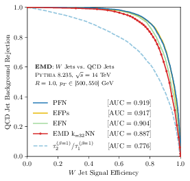
ROC curves. The red curve is the KNN with this metric, and the other curves close by are fancy ML algorithms. The light blue curve is a simple cut on N-subjettiness observables, itself an important theoretical tool

I imagine that some optimization could be done to close the small gap with respect to the best performing algorithms, for example in improving on the KNN.

The next intriguing idea presented in this paper is the fractal dimension, or correlation dimension, dim(Q), associated with their metric. The interesting bit is how dim(Q) depends on the mass/energy scale Q, which can plausibly vary from a few GeV (the regime of hadronization) up to the mass of the top quark (173 GeV). The authors compare three different sets of jets from ordinary QCD production, from W bosons decaying hadronically, and from top quarks, because one expects the detailed structure to be distinctly different, at least if viewed with the right metric. And indeed, the variation of dim(Q) with Q is quite different:

dim(Q) as a function of Q for three sources of jets

(Note these jets all have essentially the same energy.) There are at least three take-away points. First, the dim(Q) is much higher for top jets than for W and QCD jets, and W is higher than QCD. This hierarchy reflects the relative complexity of the events, and hints at new discriminating possibilities. Second, they are more similar at low scales where the structure involves hadronication, and more different at high scales which should be dominated by the decay structure. This is born out by they decay products only curves. Finally, there is little difference in the curves based on particles or on partons, meaning that the result is somehow fundamental and not an artifact of hadronization itself. I find this very exciting.

The authors develop the correlation distance dim(Q) further. It is a fact that a pair of jets from W decays boosted to the same degree can be described by a single variable: the ratio of their energies. This can be mapped onto an annulus in a abstract dimensional space (see the paper for slightly more detail). The interesting step is to look at how the complexity of individual events, reflected in dim(Q), varies around the annulus:

Embedding of W jets and how dim(Q) varies around the annulus and inside it

The blue events to the lower left are simple, with just a single round dot (jet) in the center, while the red events in the upper right have two dots of nearly equal size. The events in the center are very messy, with many dots of several sizes. So morphology maps onto location in this kinematic plane.

A second illustration is provided, this time based on QCD jets of essentially the same energy. The jet masses will span a range determined by gluon radiation and the hadronization process. Jets at lower mass should be clean and simple while jets at high mass should show signs of structure. This is indeed the case, as nicely illustrated in this picture:

How complex jet substructure correlates with jet mass

This picture is so clear it is almost like a textbook illustration.

That’s it. (There is one additional topic involving infrared divergence, but since I do not understand it I won’t try to describe it here.) The paper is short with some startling results. I look forward to the authors developing these studies further, and for other researchers to think about them and apply them to real examples.

Quark contact interactions at the LHC

So far, no convincing sign of new physics has been uncovered by the CMS and ATLAS collaborations. Nonetheless, the scientists continue to look using a wide variety of approaches. For example, a monumental work on the coupling of the Higgs boson to vector particles has been posted by the CMS Collaboration (arXiv:1411.3441). The authors conducted a thorough and very sophisticated statistical analysis of the kinematic distributions of all relevant decay modes, with the conclusion that the data for the Higgs boson are fully consistent with the standard model expectation. The analysis and article are too long for a blog post, however, so please see the paper if you want to learn the details.

The ATLAS Collaboration posted a paper on generic searches for new physics signals based on events with three leptons (e, μ and τ). This paper (arXiv:1411.2921) is longish one describing a broad-based search with several categories of events defined by lepton flavor and charge and other event properties. In all categories the observation confirms the predictions based on standard model processes: the smallest p-value is 0.05.

A completely different search for new physics based on a decades-old concept was posted by CMS (arXiv:1411.2646). We all know that the Fermi theory of weak interactions starts with a so-called contact interaction characterized by an interaction vertex with four legs. The Fermi constant serves to parametrize the interaction, and the participation of a vector boson is immaterial when the energy of the interaction is low compared to the boson mass. This framework is the starting point for other effective theories, and has been employed at hadron colliders when searching for deviations in quark-quark interactions, as might be observable if quarks were composite.

The experimental difficulty in studying high-energy quark-quark scattering is that the energies of the outgoing quarks are not so well measured as one might like. (First, the hadronic jets that materialize in the detector do not precisely reflect the quark energies, and second, jet energies cannot be measured better than a few percent.) It pays, therefore, to avoid using energy as an observable and to get the most out of angular variables, which are well measured. Following analyses done at the Tevatron, the authors use a variable χ = exp(|y₁-y₂|), which is a simple function of the quark scattering angle in the center-of-mass frame. The distribution of events in χ can be unambiguously predicted in the standard model and in any other hypothetical model, and confronted with the data. So we have a nice case for a goodness-of-fit test and pairwise hypothesis testing.

The traditional parametrization of the interaction Lagrangian is:

where the η parameters have values -1, 0, +1 and specify the chirality of the interaction; the key parameter is the mass scale Λ. An important detail is that this interaction Lagrangian can interfere with the standard model piece, and the interference can be either destructive or constructive, depending on the values of the η parameters.

The analysis proceeds exactly as one would expect: events must have at least two jets, and when there are more than two, the two highest-pT jets are used and the others ignored. Distributions of χ are formed for several ranges of di-jet invariant mass, M_JJ, which extends as high as 5.2 TeV. The measured χ distributions are unfolded, i.e., the effects of detector resolution are removed from the distribution on a statistical basis. The main sources of systematic uncertainty come from the jet energy scale and resolution and are based on an extensive parametrization of jet uncertainties.

Since one is looking for deviations with respect to the standard model prediction, it is very important to have an accurate prediction. Higher-order terms must be taken into account; these are available at next-to-leading order (NLO). In fact, even electroweak corrections are important and amount to several percent as a strong function of χ — see the plot on the right. The scale uncertainties are a few percent (again showing the a very precise SM prediction is non-trivial event for pp→2J) and fortunately the PDF uncertainties are small, at the percent level. Theoretical uncertainties dominate for M_JJ near 2 TeV, while statistical uncertainties dominate for M_JJ above 4 TeV.

The money plot is this one:

Optically speaking, the plot is not exciting: the χ distributions are basically flat and deviations due to a mass scale Λ = 10 TeV would be mild. Such deviations are not observed. Notice, though, that the electroweak corrections do improve the agreement with the data in the lowest χ bins. Loosely speaking, this improvement corresponds to about one standard deviation and therefore would be significant if CMS actually had evidence for new physics in these distributions. As far as limits are concerned, the electroweak corrections are “worth” 0.5 TeV.

The statistical (in)significance of any deviation is quantified by a ratio of log-likelihoods: q = -2ln(L_SM+NP/L_SM) where SM stands for standard model and NP for new physics (i.e., one of distinct possibilities given in the interaction Lagrangian above). Limits are derived on the mass scale Λ depending on assumed values for the η parameters; they are very nicely summarized in this graph:
The limits for contact interactions are roughly at the 10 TeV scale — well beyond the center-of-mass energy of 8 TeV. I like this way of presenting the limits: you see the expected value (black dashed line) and an envelope of expected statistical fluctuations from this expectation, with the observed value clearly marked as a red line. All limits are slightly more stringent than the expected ones (these are not independent of course).

The authors also considered models of extra spatial dimensions and place limits on the scale of the extra dimensions at the 7 TeV level.

So, absolutely no sign of new physics here. The LHC will turn on in 2015 at a significantly higher center-of-mass energy (13 TeV), and given the ability of this analysis to probe mass scales well above the proton-proton collision energy, a study of the χ distribution will be interesting.

Looking for milli-charged particles at the LHC

Andrew Haas, Chris Hill, Eder Izaguirre and Itay Yavin posted an interesting and imaginative proposal last week to search for milli-charged particles at ATLAS and CMS (arXiv:1410.6816) and I think it is worth taking a look.

Milli-charged particles can arise in some models with extra gauge bosons. The word “milli-charged” refers to the fact that the electric charge is much less than the charge of the electron. Such small charges do not arise due to some fundamental representation in the gauge theory. Rather, they arise through a (kinetic) mixing of the new gauge boson with the hyper charge field B_μ. If e’ is the charge associated with the new gauge boson and κ controls the degree of mixing, then the electric charge of the new particle ψ is ε = κe’ cosθ_W/e. The weak charge is smaller by a factor of tanθ_W. So the motivation for the search is good and the phenomenology is clear enough, and general.

A pair of hypothetical milli-charged particles would be produced through the Drell-Yan process. There are contributions from both virtual photon and Z exchange; nonetheless, the cross section is small because the charge is small. If the milli-charged particles are light enough, they can also be produced in decays of J/ψ and Υ mesons. The authors provide a plot:

Cross section for the production of a pair of milli-charged particles

Detecting a milli-charged particle is not easy because the ionization they produce as they pass through matter is much smaller than that of an electron, muon or other standard charged particle. (Recall that the ionization rate is proportional to the square of the charge of the particle.) Consequently, the trail of ions is much sparser and the amount of charge in a ionization cluster is smaller, resulting in a substantially or even dramatically reduced signal from a detector element (such as a silicon strip, proportional wire chamber or scintillator). So they cannot be reliably reconstructed as tracks in an LHC or other general-purpose detector. In fact, some searches have been done treating milli-charged particles as effectively invisible – i.e., as producing a missing energy signature. Such approaches are not effective, however, due to the large background from Z→νν.

A special detector is required and this is the crux of the Haas, Hill, Izaguirre and Yavin proposal.

This special detector must have an unusually low threshold for ionization signals. In fact, normal particles will produce relatively large signals that help reject them. Clearly, the sensitivity to very small milli-charges, ε, is determined by how low the noise level in the detector is. The main problem is that normal particles will swamp and bury any signal from milli-charged particles that may be present. One needs to somehow shield the detector from normal particles so that one can look for small-amplitude signals from milli-charged particles.

Fortunately, the main challenge of detecting milli-charged particles turns out to be a virtue: normal particles will eventually be absorbed by bulk matter – this is the principle behind the calorimeter, after all. Milli-charged particles, however, lose their energy through ionization at a much slower rate and will pass through the calorimeters with little attenuation. This is the principle of the beam-dump experiment: look for particle that are not absorbed the way the known particles are. (Implicitly we assume that the milli-charged particles have no strong interactions.)

The authors propose to install a carefully-crafted scintillator detector behind a thick wall in the CMS and/or ATLAS caverns. Typically, electronic readout devices for the normal detector are housed in a shielded room not far from the detector. This new scintillator detector would be installed inside this so-called counting room.

Schematics drawing showing how the scintillator detector would be placed in a counting room, away from the interaction point (IP)

The scintillator detector is not ordinary. It must be sensitive to rather small ionization signals which means the amplification must be large and the noise rate low. In order to fight spurious signals, the detector is divided into three parts along the flight path of the milli-charged particle and a coincidence of the three is required. In order to fight backgrounds from ordinary particles produced in the pp collisions, the detector is segmented, with each segment subtending only a very small solid angle: essentially each segment (which consists of three longitudinal pieces) forms a telescope that points narrowly at the interaction point, i.e., the origin of the milli-charged particles. Even with many such segments (“bars”), the total solid angle is miniscule so only a very small fraction of the signal would be detected – we say that the acceptance is very small. Sensitivity to the production of milli-charged particles is possible because the luminosity of the LHC will be high. Basically, the product of the cross section, the acceptance and the luminosity is a few even though the acceptance is so small. The authors estimated the reach of their experiment and produced this figure:

It is worth pointing out that this detector runs parasitically – it will not be providing triggers to the ATLAS or CMS detectors. Its time resolution should be good, about 10 ns, so it might be possible to correlate a signal from a milli-charged particle with a particular bunch crossing, but this is not really needed.

The upcoming run will be an exciting time to try this search. Evidence for milli-charged particles would be a huge discovery, of course. I do not know the status of this proposal vis-a-vis CERN and the LHC experiments. But if a signal were observed, it would clearly be easy to enhance it by building more detector. My opinion is that this is a good idea, and I hope others will agree.

The CMS kinematic edge

Does CMS observe an excess that corresponds to a signal for Supersymmetry? Opinions differ.

This week a paper appeared with the statement “…CMS has reported an intriguing excess of events with respect to the ones expected in the SM” (Huang & Wagner, arXiv:1410.4998). And last month another phenomenology paper appeared with the title “Interpreting a CMS lljjpTmiss Excess With the Golden Cascade of the MSSM” (Allanach, Raklev and Kvellestad arXiv:1409.3532). Both studies are based on a preliminary CMS report (CMS PAS SUS-12-019, Aug. 24 2014), which ends with the statement “We do not observe evidence for a statistically significant signal.”

What is going on here?

The CMS search examines the di-lepton invariant mass distribution for a set of events which have, in addition to two energetic and isolated leptons, missing transverse momentum (pTmiss) and two jets. In cascade decays of SUSY particles, χ02 → χ01 l+l-, a kind of hard edge appears at the phase space limit for the two leptons l+l-, as pointed out many years ago (PRD 55 (1997) 5520). When distinguishing a signal from background, a sharp edge is almost as good as a peak, so this is a nice way to isolate a signal if one exists. An edge can also be observed in decays of sleptons. The CMS search is meant to be as general as possible.

In order to remove the bulk of SM events producing a pair of leptons, a significant missing energy is required, as expected from a pair of neutralinos χ01. Furthermore, other activity in the event is expected (recall that there will be two supersymmetric particles in the event) so the search demands at least two jets. Hence: ll+jj+pTmiss.

A crucial feature of the analysis is motivated by the phenomenology of SUSY cascade decays: for the signal, the two leptons will have the same flavor (ee or μμ), while most of the SM backgrounds will be flavor blind (so eμ also is expected). By comparing the Mll spectrum for same-flavor and for opposite-flavor leptons, an excess might be observed with little reliance on simulations. Only the Drell-Yan background does not appear in the opposite-flavor sample at the same level as in the same-flavor sample, but a hard cut on pTmiss (also called ETmiss) removes most of the DY background. (I am glossing over careful and robust measurements of the relative e and μ reconstruction and trigger efficiencies – see the note for those details, especially Section 4.)

The CMS analyzers make an important distinction between “central” leptons with |η|<1.4 and "forward" leptons 1.6<|η|<2.4 motivated by the idea that supersymmetric particles will be centrally produced due to their high mass, and an excess may be more pronounced when both leptons are central.

A search for a kinematic edge proceed just as you would expect – a series of fits is performed with the edge placed at different points across a wide range of invariant mass Mll. The model for the Mll spectrum has three components: the flavor-symmetric backgrounds, dominated by tt, the DY background and a hypothetical signal. Both the flavor-symmetric and the DY components are described by heuristic analytical functions with several free parameters. The signal is a triangle convolved with a Gaussian to represent the resolution on Mll. Most of the model parameters are determined in fits with enhanced DY contributions, and through the simultaneous fit to the opposite-flavor sample. For the search, only three parameters are free: the signal yield in the central and forward regions and the position of the kinematic edge.

The best fitted value for the edge is y = 78.7±1.4 GeV. At that point, an excess is observed with a local statistical significance of 2.4σ, in the central region. There is no excess in the forward region. Here is the plot:

The green triangle represents the fitted signal. The red peak is, of course, the Z resonance. Here is the distribution for the forward region:

Fit to the opposite (electron-muon) invariant mass distribution

Comparing the two distributions and ignoring the Z peak, there does indeed seem to be an excess of ee and μμ pairs for Mll < 80 GeV or so. One can understand why the theorists would find this intriguing…

CMS made a second treatment of their data by defining a mass region 20 < Mll < 70 GeV and simply counting the number of events, thereby avoiding any assumptions about the shape of a signal. For this treatment, one wants to compare the data to the prediction, with suitable corrections for efficiencies, etc. Here are the plots:

By eye one can notice a tendency of the real data (dots) to fall above the prediction (solid line histogram). This tendency is much stronger for the events with two central leptons compared to the events with at least one forward lepton. Counting, CMS reports 860 observed compared to 730±40 predicted (central) and 163 observed for 157±16 forward. The significance is 2.6σ for the central di-leptons.

CMS provides a kind of teaser plot, in which they simulate three signals from the production of sbottom squarks. As you can see here, two of the models describe the apparent excess well:

Comparison to sbottom signals

So why is this not a discovery?

First of all, the statistical significance is under 3σ so formally speaking, this not even “evidence.” More importantly, the “look-elsewhere effect” has not been taken into account, as stated clearly in the CMS note. In other words, the significance for the fit is 2.4σ when you choose 78.7 GeV for the position of the edge. If you allow for any position of the edge within some wide range of Mll, then the chance that you observe an excess somewhere in that range is much greater than 1%. Similarly, the counting excess is 2.6σ for the specific box 20 < Mll < 70 GeV, but if you consider many different boxes, the chance to observe such a single excess somewhere is not so small. For this reason, the CMS Collaboration states that there is no statistically significant excess.

That said, the agreement of the simulated sbottom signals with the data is striking, even granted that there are many free parameters here that one can tune to get a good description. The Allanach et al. paper reports a scan in MSSM parameter space to find which physical SUSY parameters are consistent with the CMS data. They impose a few theoretical constraints that are not crucial at this stage, and perform a scan with simulated signals to see which ranges of parameters reproduce the CMS data and also respect constraints from other ATLAS and CMS searches. An example model is shown here:

Example spectrum from Allanach et al.

Wide ranges of sparticle masses are allowed, but there are strong constraints among them coming from the well-measured position of the edge. Constraints from (g-1)μ are respected and the relic density is good. Best of all, prospects for discovering one of these models at Run 2 are good — if such a signal really is present of course.

The Huang & Wagner paper focuses on the sbottom scenario mentioned in the CMS paper, and does a more detailed and refined analysis. They define two similar scenarios, here is the scheme for the first one:

Huang & Wagner sbottom scenario

They do not perform a scan of parameter space; rather, they select model parameters by hand to provide pertinent examples. They specifically focus on the relic density and (g-2)μ to make sure they their model can explain these facts. They explain their reasoning clearly in their paper. Their hand-tuned model does a nice job matching the CMS data. Of course, it also evades direct searches for sbottoms by both ATLAS and CMS.

What about the ATLAS 8 TeV data? For now, we must wait.

Enhanced Higgs to tau+tau- Search with Deep Learning

“Enhanced Higgs to tau+tau- Search with Deep Learning” – that is the title of a new article posted to the archive this week by Daniel Whiteson and two collaborators from the Computer Science Department at UC Irvine (1410.3469). While the title may be totally obscure to someone outside of collider physics, it caught my immediate attention because I am working on a similar project (to be released soon).

Briefly: the physics motivation comes from the need for a stronger signal for Higgs decays to τ⁺τ^–, which are important for testing the Higgs couplings to fermions (specifically, leptons). The scalar particle with a mass of 125 GeV looks very much like the standard model Higgs boson, but tests of couplings, which are absolutely crucial, are not very precise yet. In fact, indirect constraints are stronger than direct ones at the present time. So boosting the sensitivity of the LHC data to Higgs decays to fermions is an important task.

The meat of the article concerns the comparisons of shallow artificial neural networks, which contain only one or two hidden layers, and deep artificial neural networks, which have many. Deep networks are harder to work with than shallow ones, so the question is: does one really gain anything? The answer is: yes, its like increasing your luminosity by 25%.

This case study considers final states with two oppositely-charged leptons (e or μ) and missing transverse energy. The Higgs signal must be separated from the Drell-Yan production of τ pairs, especially Z→τ⁺τ^–, on a statistical basis. It appears that no other backgrounds (such as W pair or top pair production) were considered, so this study is a purely technical one. Nonetheless, there is plenty to be learned from it.

Whiteson, Baldi and Sadowski make a distinction between low-level variables, which include the basic kinematic observables for the leptons and jets, and the high-level variables, which include derived kinematic quantities such as invariant masses, differences in angles and pseudorapidity, sphericity, etc. I think this distinction and the way they compare the impact of the two sets is interesting.

The question is: if a sophisticated artificial neural network is able to develop complex functions of the low-level variables through training and optimization, isn’t it redundant to provide derived kinematic quantities as additional inputs? More sharply: does the neural network need “human assistance” to do its job?

The answer is clear: human assistance does help the performance of even a deep neural network with thousands of neurons and millions of events for training. Personally I am not surprised by this, because there is physics insight behind most if not all of the high-level variables — they are not just arbitrary functions of the low-level variables. So these specific functions carry physics meaning and fall somewhere between arbitrary functions of the input variables and brand new information (or features). I admit, though, that “physics meaning” is a nebulous concept and my statement is vague…

Comparison of the performance of shallow networks and deep networks, and also of low-level and high-level variables

The authors applied state of the art techniques for this study, including optimization with respect to hyperparameters, i.e., the parameters that concern the details of the training of the neural network (learning speed, `velocity’ and network architecture). A lot of computer cycles were burnt to carry out these comparisons!

Deep neural networks might seem like an obvious way to go when trying to isolate rare signals. There are real, non-trivial stumbling blocks, however. An important one is the vanishing gradient problem. If the number of hidden nodes is large (imagine eight layers with 500 neurons each) then training by back-propagation fails because it cannot find a significantly non-zero gradient with respect to the weights and offsets of the all the neurons. If the gradient vanishes, then the neural network cannot figure out which way to evolve so that it performs well. Imagine a vast flat space with a minimum that is localized and far away. How can you figure out which way to go to get there if the region where you are is nearly perfectly flat?

The power of a neural network can be assessed on the basis of the receiver operator curve (ROC) by integrating the area beneath the curve. For particle physicists, however, the common coinage is the expected statistical significance of an hypothetical signal, so Whiteson & co translate the performance of their networks into a discovery significance defined by a number of standard deviations. Notionally, a shallow neural network working only with low-level variables would achieve a significance of 2.57σ, while adding in the high-level variables increases the significance to 3.02σ. In contrast, the deep neural networks achieve 3.16σ with low-level, and 3.37σ with all variables.

Some conclusions are obvious: deep is better than shallow. Also, adding in the high-level variables helps in both cases. (Whiteson et al. point out that the high-level variables incorporate the τ mass, which otherwise is unavailable to the neural networks.) The deep network with low-level variables is better than a shallow network with all variables, and the authors conclude that the deep artificial neural network is learning something that is not embodied in the human-inspired high-level variables. I am not convinced of this claim since it is not clear to me that the improvement is not simply due to the inadequacy of the shallow network to the task. By way of an analogy, if we needed to approximate an exponential curve by a linear one, we would not succeed unless the range was very limited; we should not be surprised if a quadratic approximation is better.

In any case, since I am working on similar things, I find this article very interesting. It is clear that the field is moving in the direction of very advanced numerical techniques, and this is one fruitful direction to go in.

Neural Networks for Triggering

As experiments push the high-energy frontier, and also the intensity frontier, they must contend with higher and higher instantaneous luminosities. This challenge drives experimenters to try new techniques for triggering that might have sounded outlandish or fanciful ten years ago.

The Belle II experiment posted a paper this week on using (artificial) neural networks at the first trigger level for their experiment (arXiv:1410.1395). To be explicit: they plan to implement an artificial neural network at the hardware-trigger level, L1, i.e., the one that deals with the most primitive information from the detector in real time. The L1 latency is 5 μs which allows only 1 μs for the trigger decision.

At issue is a major background coming from Touschek scattering. The coulomb interaction of the e- and e+ beams can transform a small transverse phase space into a long longitudinal phase space. (See a DESY report 98-179 for a discussion.) The beam is thereby spread out in the z direction leading to collisions taking place far from the center of the apparatus. This is a bad thing for analysis and for triggering since much of the event remains unreconstructed — such events are a waste of bandwidth. The artificial neural networks, once trained, are mechanistic and parallel in the way they do their calculations, therefore they are fast – just what is needed for this situation. The interesting point is that here, in the Belle application, decisions about the z position of the vertex will be made without reconstructing any tracks (because there is insufficient time to carry out the reconstruction).

The CDC has 56 axial and stereo layers grouped into nine superlayers. Track segments are found by the TSF based on superlayer information. The 2D trigger module finds crude tracks in the (r,φ) plane. The proposed neutral network trigger takes information from the axial and stereo TSF, and also from the 2D trigger module.

Diagram of the Belle trigger.

As usual, the artificial neural network is based on the multi-layer perceptron (MLP) with a hyperbolic tangent activation function. The network is trained by back-propagation. Interestingly, the authors use an ensemble of “expert” MLPs corresponding to small sectors in phase space. Each MLP is trained on a subset of tracks corresponding to that sector. Several incarnations of the network were investigated, which differ in the precise information used as input to the neural network. The drift times are scaled and the left/right/undecided information is represented by an integer. The azimuthal angle can be represented by a scaled wire ID or by an angle relative to the one produced by the 2D trigger. There is a linear relation between the arc length and the z coordinate, so the arc length (μ) can also be a useful input variable.

As a first test, one sector is trained for a sample of low-pT and another sample of high-pT tracks. The parameter range is very constrained, and the artificial neural networks do well, achieving a resolution of 1.1 – 1.8 cm.

In a second test, closer to the planned implementation, the output of the 2D trigger is represented by some smeared φ and pT values. The track parameters cover a wider range than in the first test, and the pT range is divided into nine pieces. The precision is 3 – 7cm in z, which is not yet good enough for the application (they are aiming for 2 cm or better). Nonetheless, this estimate is useful because it can be used to restrict the sector size for the next step.

Resolution on z versus curvature, for three versions of the neural network.

Clearly this is a work in progress, and much remains to be done. Assuming that the Belle Collaboration succeeds, the fully pipelined neural network trigger will be realized on FPGA boards.

LHCb searches for LFV in tau decays

Lepton flavor violation (LFV) occurs when neutrinos oscillate in flavor, but is not supposed to occur (at tree level) when charged leptons are involved. Beyond the standard model, however, speculative models predict observable levels of LFV and since flavor is so difficult to understand theoretically, searches for LFV are inherently worthwhile.

A striking signature for LFV would be the neutrinoless decay of a tau lepton to three muons (or, for that matter, the decay of a muon to three electrons). The Belle and BaBar experiments at the B-factories have searched for τ→3μ; Belle set the best limit in 2010: BF(τ→3μ) < 2.1×10^-8.

Tau leptons are produced copiously in high-energy pp collisions. They come from the semileptonic decays of b and c hadrons, which themselves are produced with huge cross sections. The LHCb experiment is designed to study b and c hadrons and is very successful at that. A key piece of the LHCb apparatus is a very nice muon spectrometer that provides triggers for the readout and a high-quality reconstruction of muon trajectories. This would seem to be an excellent place to search for τ→3μ decays – and it is, as reported this week (arXiv:1409.8548).

The selection begins, of course, with three muons that together form a displaced vertex (taking advantage of the tau and charm hadron lifetimes). The momentum vector of the three muons should be nearly collinear with a vector pointing from the primary vertex to the tri-muon vertex — there are no neutrinos in the signal, after all, and the tau lepton takes most of the energy of the charm hadron, and therefore closely follows the direction of the charm hadron. (Charm hadron decays produce most of the tau leptons, so those coming from b hadrons are lost, but this does not matter much.) Here is a depiction of a signal event, which comes from a talk given by Gerco Onderwater at NUFACT2014:

I like the way the analysis is designed: there is the all-important tri-muon invariant mass distribution, there is a classifier for “geometry” – i.e., topology, and a second one for muon identification. Clearly, this analysis is challenging.

The geometry classifier M(3body) incorporates information about the vertex and the pointing angle. The classifier itself is surprisingly sophisticated, involving two Fisher discriminants, four artificial neural networks, one function-discriminant analysis and one linear discriminant — all combined into a blended boosted decision tree (BDT)! Interestingly, the analyzers use one-half of their event sample to train the artificial neural networks, etc., and the other to train the BDT. The performance of the BDT is validated with a sample of Ds→φπ decays, with φ→2μ.

The muon ID classifier M(PID) uses detector information from the ring-imaging cherenkov detectors, calorimeters and muon detectors to provide a likelihood that each muon candidate is a muon. The smallest of the three likelihoods is used as the discriminating quantity. M(PID) employs an artificial neural network that is validated using J/ψ decays to muon pairs.

The LHCb physicists take advantage of their large sample of Ds→μμπ decays to model the tri-muon invariant mass distribution accurately. The line shape is parameterized by a pair of Gaussians that are then rescaled to the mass and width of the tau lepton.

Backgrounds are not large, and consist of one irreducible background and several reducible ones, which is where M(PID) plays a key role. The signal rate is normalized to the rate of Ds→φπ decays, which is relatively well known, and which also has a robust signal in LHCb.

The paper contains tables of yields in grids of M(PID) and M(3body), and there is no signs of a signal. The picture from their Fig. 3 is clear:

LHCb trimuon spectra

No signal. Taking relatively modest systematics into account, they use the usual CLs method to set an upper limit. The actual result is BF(τ→3μ) < 4.6×10^-8 at 90% CL, slightly better than expected. This limit is not quite as constraining as the earlier Belle result, but points the way to stronger results when larger data samples have been collected. The mass window shown above is not heavily populated by background.

I think this is a nice analysis, done intelligently. I hope I can learn more about the advanced analysis techniques employed.

CMS resolves states with a mass difference of 19 MeV

This week the CMS Collaboration released a paper reporting the measurement of the ratio of production cross sections for the χb2(1P) and the χb1(1P) heavy meson states (arXiv:1409.5761). The motivation stems from the theoretical difficulties in explaining how such states are formed, but for me as an experimenter the most striking feature of the analysis is the impressive separation of the χ states.

First, a little background. A bottom quark and an anti-bottom anti-quark can form a meson with a well-defined mass. These states bear some resemblance to positronium but the binding potential comes from the strong force, not electromagnetism. In the past, the spectrum of the masses of these states clarified important features of this potential, and led to the view that the potential increases with separation, rather than decreasing. As we all know, QCD is absolutely confining, and the first hints came from studies of charmonium and bottomonium. The masses of these and many other states have been precisely measured over the years, and now provide important tests of lattice calculations.

The mass of the χb2(1P) is 9912.21 MeV and the mass of the χb1(1P) is 9892.78 MeV; the mass difference is only 19.4 MeV. They sit together in a fairly complicated diagram of the states. Here is a nice version which comes from an annual review article by Patrignani, Pedlar and Rosner (arXiv:1212.6552) – I have circled the states under discussion here:

Bottomonium states

So, even on the scale of the bottomonium mesons, this separation of 19 MeV is quite small. Nonetheless, CMS manages to do a remarkably good job. Here is their plot:

Reconstructed chi states

Two peaks are clearly resolved: the χb2(1P) on the left (and represented by the green dashed line) and the χb1(1P) on the right (represented by the red dashed line). The two peaks are successfully differentiated, and the measurements of their relative rates can be carried out.

How do they do it? The χ stated decay to the Y(1S) by emitting a photon with a substantial branching fraction that is already known fairly well. The vector Y(1S) state is rather easily reconstructed through through its decays to a μ+μ- pair. The CMS spectrometer is excellent, as it the reconstruction of muons, so the Y(1S) state appears as a narrow peak. By detecting the photon and calculating the μμγ invariant mass, the χ states can be reconstructed.

Here is the interesting part: the photons are not reconstructed with the (rather exquisite) crystal electromagnetic calorimeter, because its energy resolution is not good enough. This may be surprising, since the Higgs decay to a pair of photons certainly is well reconstructed using the calorimeter. These photons, however, have a very low energy, and their energies are not so well measured. (Remember that electromagnetic calorimeter resolution goes roughly as 1/sqrt(E).) Instead, the CMS physicists took advantage of their tracking a second time, and reconstructed those photons that had cleanly converted into an e+e- pair. So the events of interest contained two muons, that together give the Y(1S) state, and an e+e- pair, which gives the photon emitted in the radiative decay of the χ state. The result is the narrow peaks displayed above; the yield is obtained simply by integrating the curves representing the two χ states.

This technique might conceivably be interesting when searching for peculiar signals of new physics.

It is difficult to ascertain the reconstruction efficiency of conversion pairs, since they tend to be asymmetric (either the electron or the positron gets most of the photon’s energy). By taking the ratio of yields, however, one obtains the ratio of cross sections times branching fractions. This ratio is experimentally clean, therefore, and robust. The mass spectrum was examined in four bins of the transverse momentum of the Y(1S); the plot above is the second such bin.

Here is the results of the measurement: four values of the ratio σ(χb2)/σ(χb1) plotted as a function of p_T(Y):

Ratio of cross sections

LHCb have also made this measurement (arXiv:1202.1080), and their values are presented by the open circles; the CMS measurement agrees well with LHCb. The green horizontal band is simply an average of the CMS values, assuming no dependence on p_T(Y). The orange curved band comes from a very recent theoretical calculation by Likhoded, Luchinsky and Poslavsky (arXiv:1409.0693). This calculation does not reproduce the data.

I find it remarkable that the CMS detector (and the other LHC detectors to varying degrees) can resolve such a small mass difference when examining the debris from an 8 TeV collision. These mass scales are different by a factor of two million. While there is no theoretical significance to this fact, it shows that experimenters must and can deal with such a huge range within one single apparatus. And they can.

New AMS Results – hints of TeV Dark Matter?

Yesterday the AMS Collaboration released updated results on the positron excess. The press release is available at the CERN press release site. (Unfortunately, the AMS web site is down due to syntax error – I’m sure this will be fixed very soon.)

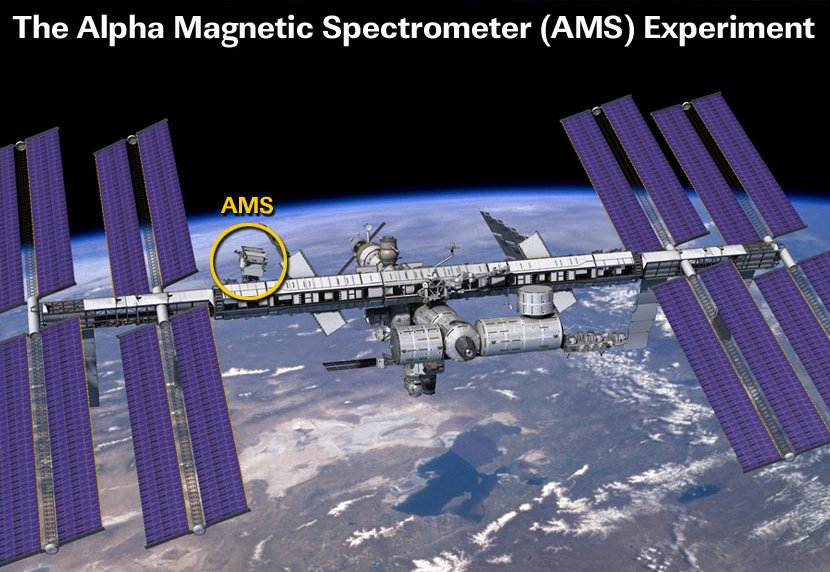
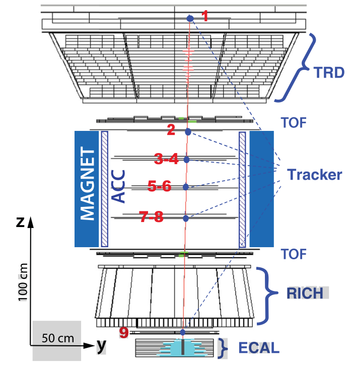
The Alpha Magnetic Spectrometer was installed three years ago at the International Space Station. As the name implies, it can measure the charge and momenta of charged particles. It can also identify them thanks to a suite of detectors providing redundant and robust information. The project was designed and developed by Prof. Sam Ting (MIT) and his team. An international team including scientists at CERN coordinate the analysis of data.

There are more electrons than positrons striking the earth’s atmosphere. Scientists can predict the expected rate of positrons relative to the rate of electrons in the absence of any new phenomena. It is well known that the observed positron rate does not agree with this prediction. This plot shows the deviation of the AMS positron fraction from the prediction. Already at an energy of a couple of GeV, the data have taken off.

AMS positron fraction compared to prediction.

The positron fraction unexpectedly increases starting around 8 GeV. At first it increases rapidly, with a slower increase above 10 GeV until 250 GeV or so. AMS reports the turn-over to a decrease to occur at 275 ± 32 GeV though it is difficult to see from the data:

AMS positron fraction. The upper plot shows the slope.

This turnover, or edge, would correspond notionally to a Jacobian peak — i.e., it might indirectly indicate the mass of a decaying particle. The AMS press release mentions dark matter particles with a mass at the TeV scale. It also notes that no sharp structures are observed – the positron fraction may be anomalous but it is smooth with no peaks or shoulders. On the other hand, the observed excess is too high for most models of new physics, so one has to be skeptical of such a claim, and think carefully for an astrophysics origin of the “excess” positrons — see the nice discussion in Resonaances.

As an experimenter, it is a pleasure to see this nice event display for a positron with a measured energy of 369 GeV:

AMS event display: a high-energy positron

Finally, AMS reports that there is no preferred direction for the positron excess — the distribution is isotropic at the 3% level.

There is no preprint for this article. It was published two days ago in PRL 113 (2014) 121101″