The CMS kinematic edge

Does CMS observe an excess that corresponds to a signal for Supersymmetry? Opinions differ.

This week a paper appeared with the statement “…CMS has reported an intriguing excess of events with respect to the ones expected in the SM” (Huang & Wagner, arXiv:1410.4998). And last month another phenomenology paper appeared with the title “Interpreting a CMS lljjpTmiss Excess With the Golden Cascade of the MSSM” (Allanach, Raklev and Kvellestad arXiv:1409.3532). Both studies are based on a preliminary CMS report (CMS PAS SUS-12-019, Aug. 24 2014), which ends with the statement “We do not observe evidence for a statistically significant signal.”

What is going on here?

The CMS search examines the di-lepton invariant mass distribution for a set of events which have, in addition to two energetic and isolated leptons, missing transverse momentum (pTmiss) and two jets. In cascade decays of SUSY particles, χ02 → χ01 l+l-, a kind of hard edge appears at the phase space limit for the two leptons l+l-, as pointed out many years ago (PRD 55 (1997) 5520). When distinguishing a signal from background, a sharp edge is almost as good as a peak, so this is a nice way to isolate a signal if one exists. An edge can also be observed in decays of sleptons. The CMS search is meant to be as general as possible.

In order to remove the bulk of SM events producing a pair of leptons, a significant missing energy is required, as expected from a pair of neutralinos χ01. Furthermore, other activity in the event is expected (recall that there will be two supersymmetric particles in the event) so the search demands at least two jets. Hence: ll+jj+pTmiss.

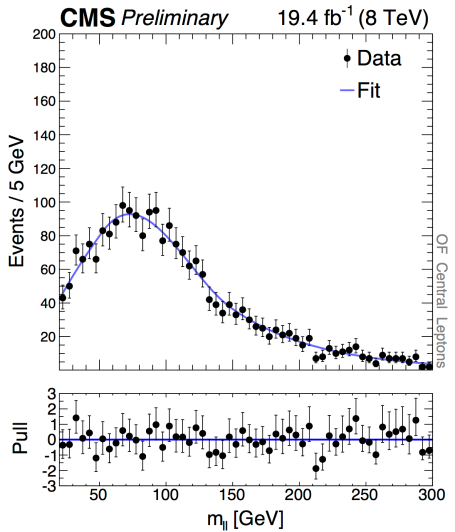
A crucial feature of the analysis is motivated by the phenomenology of SUSY cascade decays: for the signal, the two leptons will have the same flavor (ee or μμ), while most of the SM backgrounds will be flavor blind (so eμ also is expected). By comparing the Mll spectrum for same-flavor and for opposite-flavor leptons, an excess might be observed with little reliance on simulations. Only the Drell-Yan background does not appear in the opposite-flavor sample at the same level as in the same-flavor sample, but a hard cut on pTmiss (also called ETmiss) removes most of the DY background. (I am glossing over careful and robust measurements of the relative e and μ reconstruction and trigger efficiencies – see the note for those details, especially Section 4.)

The CMS analyzers make an important distinction between “central” leptons with |η|<1.4 and "forward" leptons 1.6<|η|<2.4 motivated by the idea that supersymmetric particles will be centrally produced due to their high mass, and an excess may be more pronounced when both leptons are central.

A search for a kinematic edge proceed just as you would expect – a series of fits is performed with the edge placed at different points across a wide range of invariant mass Mll. The model for the Mll spectrum has three components: the flavor-symmetric backgrounds, dominated by tt, the DY background and a hypothetical signal. Both the flavor-symmetric and the DY components are described by heuristic analytical functions with several free parameters. The signal is a triangle convolved with a Gaussian to represent the resolution on Mll. Most of the model parameters are determined in fits with enhanced DY contributions, and through the simultaneous fit to the opposite-flavor sample. For the search, only three parameters are free: the signal yield in the central and forward regions and the position of the kinematic edge.

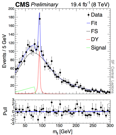
The best fitted value for the edge is y = 78.7±1.4 GeV. At that point, an excess is observed with a local statistical significance of 2.4σ, in the central region. There is no excess in the forward region. Here is the plot:

The green triangle represents the fitted signal. The red peak is, of course, the Z resonance. Here is the distribution for the forward region:

Fit to the opposite (electron-muon) invariant mass distribution

Comparing the two distributions and ignoring the Z peak, there does indeed seem to be an excess of ee and μμ pairs for Mll < 80 GeV or so. One can understand why the theorists would find this intriguing…

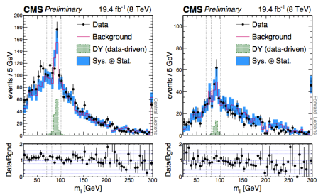
CMS made a second treatment of their data by defining a mass region 20 < Mll < 70 GeV and simply counting the number of events, thereby avoiding any assumptions about the shape of a signal. For this treatment, one wants to compare the data to the prediction, with suitable corrections for efficiencies, etc. Here are the plots:

By eye one can notice a tendency of the real data (dots) to fall above the prediction (solid line histogram). This tendency is much stronger for the events with two central leptons compared to the events with at least one forward lepton. Counting, CMS reports 860 observed compared to 730±40 predicted (central) and 163 observed for 157±16 forward. The significance is 2.6σ for the central di-leptons.

CMS provides a kind of teaser plot, in which they simulate three signals from the production of sbottom squarks. As you can see here, two of the models describe the apparent excess well:

Comparison to sbottom signals

So why is this not a discovery?

First of all, the statistical significance is under 3σ so formally speaking, this not even “evidence.” More importantly, the “look-elsewhere effect” has not been taken into account, as stated clearly in the CMS note. In other words, the significance for the fit is 2.4σ when you choose 78.7 GeV for the position of the edge. If you allow for any position of the edge within some wide range of Mll, then the chance that you observe an excess somewhere in that range is much greater than 1%. Similarly, the counting excess is 2.6σ for the specific box 20 < Mll < 70 GeV, but if you consider many different boxes, the chance to observe such a single excess somewhere is not so small. For this reason, the CMS Collaboration states that there is no statistically significant excess.

That said, the agreement of the simulated sbottom signals with the data is striking, even granted that there are many free parameters here that one can tune to get a good description. The Allanach et al. paper reports a scan in MSSM parameter space to find which physical SUSY parameters are consistent with the CMS data. They impose a few theoretical constraints that are not crucial at this stage, and perform a scan with simulated signals to see which ranges of parameters reproduce the CMS data and also respect constraints from other ATLAS and CMS searches. An example model is shown here:

Example spectrum from Allanach et al.

Wide ranges of sparticle masses are allowed, but there are strong constraints among them coming from the well-measured position of the edge. Constraints from (g-1)μ are respected and the relic density is good. Best of all, prospects for discovering one of these models at Run 2 are good — if such a signal really is present of course.

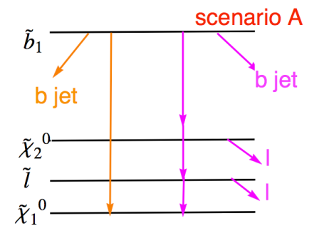
The Huang & Wagner paper focuses on the sbottom scenario mentioned in the CMS paper, and does a more detailed and refined analysis. They define two similar scenarios, here is the scheme for the first one:

Huang & Wagner sbottom scenario

They do not perform a scan of parameter space; rather, they select model parameters by hand to provide pertinent examples. They specifically focus on the relic density and (g-2)μ to make sure they their model can explain these facts. They explain their reasoning clearly in their paper. Their hand-tuned model does a nice job matching the CMS data. Of course, it also evades direct searches for sbottoms by both ATLAS and CMS.

What about the ATLAS 8 TeV data? For now, we must wait.